Numerical Computing with NumPy

NumPy (short for Numerical Python) is an open-source Python library widely used in scientific computing—particularly for array operations, linear algebra, Fourier transforms, and random number generation. It provides a powerful N-dimensional array object along with a comprehensive set of functions for manipulating these arrays. Many advanced scientific computing libraries, such as Pandas and Matplotlib, are built on top of NumPy.

Installation

NumPy is a third-party package. If you haven't installed it yet, you can do so using pip:

pip install numpy

To use NumPy, you first need to import it:

import numpy as np

Note: Some import statements are omitted in the examples below. Be sure to import numpy as np when testing them.

Arrays

At the core of NumPy is the N-dimensional array (ndarray) object, which serves as a fast and flexible container for large datasets. Compared to Python's built-in lists, NumPy arrays are significantly more efficient and support advanced mathematical operations. Here are some of the most common array operations:

Creating Arrays

Use the np.array() function to convert Python sequences (like lists) into NumPy arrays:

# Convert a list to an array
np_array = np.array([1, 2, 3, 4, 5])

# Convert an image to a two-dimensional array
from PIL import Image
image = Image.open("example.jpg")
image_array = np.array(image)

Use np.zeros() and np.ones() to create arrays prefilled with zeros or ones of a specified shape:

zeros_array = np.zeros((2, 3))  # Create a 2x3 zero matrix
ones_array = np.ones((3, 4))    # Create a 3x4 matrix of ones
range_array = np.arange(10)     # Create an array with values from 0 to 9
random_array = np.random.randint(0, 10, (3, 4))  # Create a 3x4 matrix with random integers from 0 to 9

Array Shape and Size

The shape attribute describes the dimensions of an array:

import numpy as np
ones_array = np.ones((3, 4)) 
print(ones_array.shape)         # Output: (3, 4)

reshape can change the shape of an array without modifying its data:

import numpy as np

# Create a one-dimensional array
arr = np.arange(10)  # This creates an array containing numbers 0 through 9
print("Original array:")
print(arr)

# Use reshape to rearrange it into a 2x5 two-dimensional array
reshaped_arr = arr.reshape((2, 5))
print("\nReshaped two-dimensional array:")
print(reshaped_arr)

# You can also let NumPy automatically compute one of the dimensions
# The -1 below means automatically calculate that dimension's size
reshaped_arr_2 = arr.reshape((5, -1))
print("\nReshaped array with auto-computed dimension:")
print(reshaped_arr_2)

Output:

Original array:
[0 1 2 3 4 5 6 7 8 9]

Reshaped two-dimensional array:
[[0 1 2 3 4]
 [5 6 7 8 9]]

Reshaped array with auto-computed dimension:
[[0 1]
 [2 3]
 [4 5]
 [6 7]
 [8 9]]

Indexing and Slicing

Indexing a one-dimensional NumPy array works exactly like indexing a standard Python list:

element = np_array[0]  # Get the first element

However, multi-dimensional arrays use a comma-separated tuple for indexing. For a two-dimensional array (matrix), the syntax is array[row, column]:

# Create a 3x3 two-dimensional array
arr = np.array([[1, 2, 3], [4, 5, 6], [7, 8, 9]])

# Access the element at the second row and third column
print(arr[1, 2])  # Output: 6

NumPy arrays also support slicing, following the same rules as list slicing:

# Access the second row
print(arr[1, :])  # Output: [4 5 6]

# Access the third column
print(arr[:, 2])  # Output: [3 6 9]

# Access a sub-matrix (first two rows, first two columns)
print(arr[:2, :2])  # Output: [[1 2] [4 5]]

NumPy also supports integer array indexing, which allows you to select arbitrary elements using other arrays as indices:

print(arr[[0, 2], [1, 2]])  
# Output: [2 9]  i.e., indexing two elements: arr[0, 1] and arr[2, 2]

Boolean Indexing (Conditional Selection)

NumPy also supports boolean indexing, which allows you to filter or select elements based on logical conditions:

# Create a boolean array indicating which elements are greater than 5
bool_idx = arr > 5

# Index using the boolean array
print(arr[bool_idx])  # Output: [6 7 8 9]

This feature is incredibly useful for updating elements that meet specific criteria.

For example, to change all elements less than zero to zero:

import numpy as np

# Create an example array
arr = np.array([1, -2, 3, -4, 5])

# Change all elements less than zero to zero
arr[arr < 0] = 0

You can also modify elements in one array based on a condition applied to another array of the same shape:

import numpy as np

# Create two example arrays
arr1 = np.array([1, 2, 3, 4, 5])
arr2 = np.array([5, 4, 3, 2, 1])

# Modify elements in arr1 based on a condition in arr2 (e.g., elements less than 3)
condition = arr2 < 3  # Condition: elements in arr2 less than 3
arr1[condition] = 0  # Set elements in arr1 to 0 where the corresponding condition in arr2 is True

Matrix Operations

NumPy provides a vast library of mathematical functions. In this section, we will focus on the most fundamental operations: basic matrix math.

Arithmetic Operations

The most common arithmetic operations are addition, subtraction, multiplication, and division:

import numpy as np

# Create two matrices
A = np.array([[1, 2], [3, 4]])
B = np.array([[5, 6], [7, 8]])

# Matrix addition
addition = A + B
print("Matrix addition A + B:\n", addition)

# Matrix subtraction
subtraction = A - B
print("\nMatrix subtraction A - B:\n", subtraction)

# Element-wise multiplication
elementwise_multiplication = A * B
print("\nElement-wise multiplication A * B:\n", elementwise_multiplication)

# Dot product (matrix multiplication)
dot_product = np.dot(A, B)
print("\nDot product A dot B:\n", dot_product)

# Element-wise division
elementwise_division = A / B
print("\nElement-wise division A / B:\n", elementwise_division)

Output:

Matrix addition A + B:
 [[ 6  8]
 [10 12]]

Matrix subtraction A - B:
 [[-4 -4]
 [-4 -4]]

Element-wise multiplication A * B:
 [[ 5 12]
 [21 32]]

Dot product A dot B:
 [[19 22]
 [43 50]]

Element-wise division A / B:
 [[0.2        0.33333333]
 [0.42857143 0.5       ]]

Axis Operations

When working with multi-dimensional arrays, you often need to perform calculations along specific dimensions (referred to as axes), such as computing sums, means, or maximums. Here are some examples of axis-based calculations:

import numpy as np

# Create a 3x3 matrix
matrix = np.array([[1, 2, 3], [4, 5, 6], [7, 8, 9]])

# Compute the sum of all elements
total_sum = np.sum(matrix)
print("Sum of all matrix elements:", total_sum)

# Compute the sum of each column
col_sum = np.sum(matrix, axis=0)
print("Sum of each column:", col_sum)

# Compute the sum of each row
row_sum = np.sum(matrix, axis=1)
print("Sum of each row:", row_sum)

# Compute the average of each column
col_mean = np.mean(matrix, axis=0)
print("Average of each column:", col_mean)

# Compute the average of each row
row_mean = np.mean(matrix, axis=1)
print("Average of each row:", row_mean)

# Compute the maximum of each column
col_max = np.max(matrix, axis=0)
print("Maximum of each column:", col_max)

# Compute the maximum of each row
row_max = np.max(matrix, axis=1)
print("Maximum of each row:", row_max)

Linear Algebra Operations

Matrix multiplication, inversion, etc.

import numpy as np

# Create two matrices
A = np.array([[1, 2, 3], [4, 5, 6], [7, 8, 9]])
B = np.array([[9, 8, 7], [6, 5, 4], [3, 2, 1]])

# Matrix transpose
transpose_A = A.T
transpose_B = B.T

# Try to compute the inverse of matrix A (if possible)
try:
    inverse_A = np.linalg.inv(A)
except np.linalg.LinAlgError:
    inverse_A = "Not invertible"

# Print results
print("Matrix A:\n", A)
print("Matrix B:\n", B)
print("Transpose of A:\n", transpose_A)
print("Transpose of B:\n", transpose_B)
print("Inverse of A:\n", inverse_A)

Fast Fourier Transform

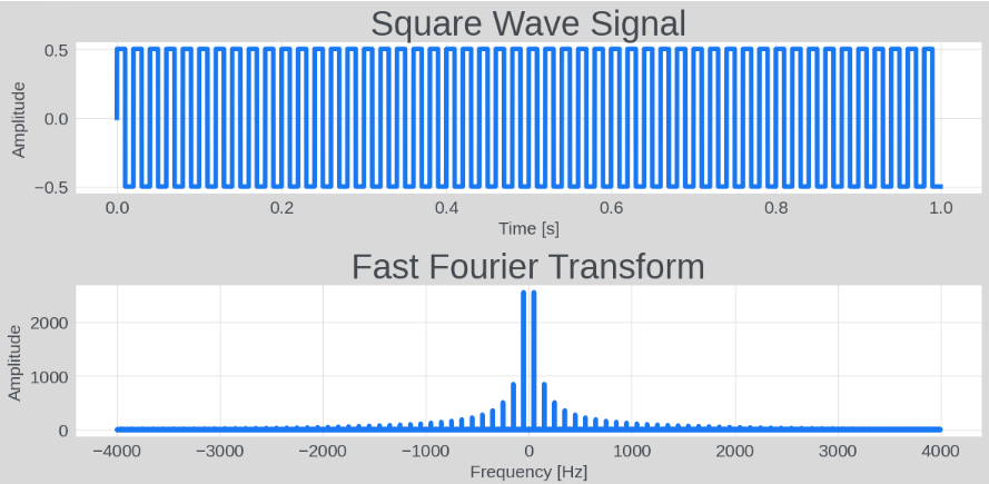
The Fast Fourier Transform (FFT) converts signals between the time domain and the frequency domain. It is widely used in signal processing, image analysis, audio processing, and engineering.

import numpy as np
import matplotlib.pyplot as plt

# Create a square wave signal
Fs = 8000   # Sampling frequency
f = 50      # Signal frequency
t = np.linspace(0, 1, Fs, endpoint=False)  # Time axis
# signal = 0.5 * np.sin(2 * np.pi * f * t)  # Generate a sine wave
signal = 0.5 * np.sign(np.sin(2 * np.pi * f * t))  # Generate a square wave

# Fast Fourier Transform
fft_result = np.fft.fft(signal)
fft_freq = np.fft.fftfreq(t.shape[-1], d=1/Fs)

# Plot
plt.figure(figsize=(12, 6))

# Plot the original signal
plt.subplot(2, 1, 1)
plt.plot(t, signal)
plt.title('Square Wave Signal')
plt.xlabel('Time [s]')
plt.ylabel('Amplitude')

# Plot the FFT result
plt.subplot(2, 1, 2)
plt.plot(fft_freq, np.abs(fft_result))
plt.title('Fast Fourier Transform')
plt.xlabel('Frequency [Hz]')
plt.ylabel('Amplitude')

plt.tight_layout()
plt.show()

Result:

Array Broadcasting

Broadcasting allows NumPy to perform arithmetic operations on arrays of different shapes, automatically expanding the smaller array to match the larger one without copying data.

Broadcasting Rules

Broadcasting follows a strict set of rules:

1. Dimension Matching: If the two arrays differ in their number of dimensions, the shape of the lower-dimensional array is padded with ones on its left side.
2. Size Compatibility: If the sizes of the arrays differ in a dimension, but one of them is 1, that array is conceptually stretched (without copying data) to match the size of the other.
3. Mismatch Error: If the sizes differ in any dimension and neither is 1, a ValueError is raised.

Addition

Suppose we add a 2x3 array A and a 1x3 array B. B is broadcast along the vertical axis to match the shape of A before addition:

A = np.array([[1, 2, 3], [4, 5, 6]])
B = np.array([1, 2, 3])

# B will be "expanded" along the first dimension to match A's shape
C = A + B

# Result: C = [[2, 4, 6], [5, 7, 9]]

Multiplication

Suppose we multiply a 3x1 array A by a scalar B. B is broadcast to match A's shape:

A = np.array([[1], [2], [3]])
B = 2

# B is broadcast to 3x1, then multiplied with A
C = A * B

# Result: C = [[2, 4, 6]]

Advantages and Disadvantages

Broadcasting makes code more readable and computationally efficient by eliminating the need to write loops or manually copy data. NumPy performs the broadcast operations in optimized C under the hood.

However, misapplying these rules can lead to subtle bugs or unexpected output. When working with multi-dimensional data, always verify the shapes of your arrays to ensure they broadcast as expected.

Rich Numerical Types

To support high-performance scientific computing, NumPy offers a much wider range of numerical data types than Python's built-in types. Their names indicate their precision and representation: for example, np.int8 represents an 8-bit signed integer (from -128 to 127), np.uint64 is a 64-bit unsigned integer, and np.float16 is a half-precision floating-point number.

When using NumPy, you can usually let NumPy automatically select the most appropriate data type. However, when optimizing memory usage or ensuring numerical precision, you can also explicitly specify which type to use. For example:

arr = np.array([1, 2, 3], dtype=np.float32)  # Create an array of type float32

Choosing the correct data type is critical for optimizing memory and computation speed when working with massive datasets. For example, deep learning models often use np.float16 to reduce memory bandwidth demands during training.

Syntax Placeholders and the Ellipsis

In Python, you sometimes need placeholders to write syntactically valid code for blocks you plan to implement later, or to discard unused values.

Underscore

The underscore _ is conventionally used to denote a throwaway variable. For example, in loops where the loop variable is not used, or when unpacking sequences where some elements are ignored:

# Perform some operation for each element in a list, but you don't actually need the element itself
for _ in range(5):
    print("Execute repeatedly")

# Ignore certain values during unpacking
a, _, b = (1, 2, 3)  # a = 1, b = 3

pass

We have used pass frequently. It is a null statement used when syntax requires a statement but no action is needed. It is ideal for sketching out unimplemented functions, classes, or control flow blocks:

def my_func():
    pass

print(my_func())

Because a Python function body cannot be completely empty, pass serves as a placeholder until the actual logic is written.

Ellipsis

Python also has a more convenient placeholder: three dots: .... For example:

def my_func():
    ...

print(my_func())

The effect is the same as using pass. However, they also differ: pass is a statement, while ... is a special value. You cannot write return pass, but you can write return ...:

def my_func():
    return ...

print(my_func())  # Output: Ellipsis

Running the code above prints Ellipsis. In addition to serving as a placeholder, Ellipsis is a built-in singleton value in Python. Its most powerful application is in multi-dimensional array slicing, where it represents an arbitrary number of full-slice (:) dimensions. For example:

import numpy as np

# Create a four-dimensional array with shape 2*3*4*5, total 120 elements
arr = np.arange(120).reshape(2, 3, 4, 5)

# Use Ellipsis to select all elements, equivalent to arr[:, :, :, :]
print(arr[...])   # Prints the entire four-dimensional array, data from 0 to 119

# Use Ellipsis to select all elements with index 0 in the last dimension, equivalent to arr[:, :, :, 0]
print(arr[..., 0])

# Output:
# [[[  0   5  10  15]
#   [ 20  25  30  35]
#   [ 40  45  50  55]]
# 
#  [[ 60  65  70  75]
#   [ 80  85  90  95]
#   [100 105 110 115]]]


# Use Ellipsis to select all elements with index 1 in the first and last dimensions, equivalent to arr[1, :, :, 1]
print(arr[1, ..., 0])

# Output:
# [[ 60  65  70  75]
#  [ 80  85  90  95]
#  [100 105 110 115]]

Because ... dynamically replaces an arbitrary number of dimensions, you can use at most one ellipsis in a single slicing expression to avoid ambiguity.